The whys and hows of data preparation is a series of blog posts explaining the importance of data nowadays and how it can be processed to extract as much value as possible, you can find the first post of the series here and the second one here.

In the previous posts we gave a multifold overview of the concept of data preprocessing. First we defined it as that series of processes designed to transform raw data into good quality data, then we analysed some of the most common techniques in this field. Now it's time to get your hands dirty with some code. We recently released a small open source library, where we implemented a "mini" version of a preprocessor for tabular data.

Solution design

As mentioned, this is a "mini" version of a data preprocessor, usable for educational purposes and small projects. First of all, for simplicity, we treated only two possible types of features, the same ones seen in previous articles: numerical and categorical. In real cases, other types of features may be encountered, such as temporal or boolean ones. For example, as we will see later, our preprocessor considers these features as numeric. As for the transformations used, we made arbitrary choices and used the most common ones.

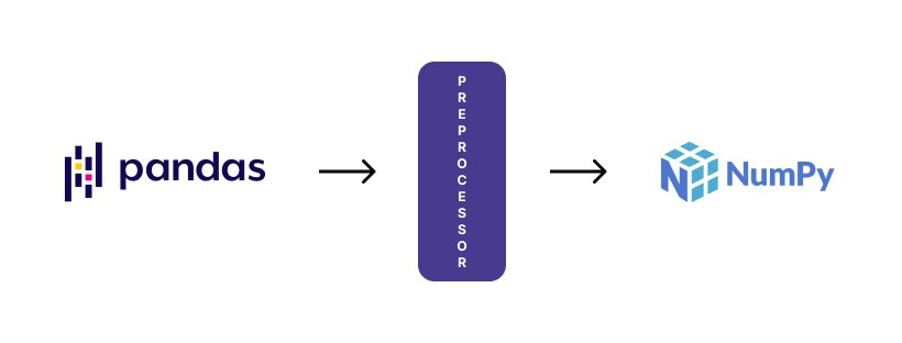
Finally, another important decision in the implementation concerned both the format for the input data and for the output of our preprocessing pipeline. For our library we focused on the most common formats for tabular data. In particular, the raw data received, in the form of a csv file, is read as a Pandas DataFrame. The data returned by the preprocessor instead takes the form of a Numpy Ndarray.

What if those decisions aren't right for your project? Or if they are not enough for your needs? Well, that’s the beauty and power of open source software, isn’t it? Fork and remix the code however you like! We will be happy to see your personal implementation.

Implementation

The first operation to perform in order to use our preprocessor is to instantiate it and train it to recognise and transform a certain type of data. In order to instantiate an object, first we need to pass a DataFrame with the raw data to it. At this point, two fundamental steps for the process take place in the initialization:

• We carry out the inference of the column type, dividing between numeric and categorical features;
• We select the features we will use, discarding those that do not carry significant information.

After these two operations, it is possible to define the transformation pipeline for our data.

Column types inference

def _infer_feature_types(self, data: pd.DataFrame) -> None:
       boolean_features = list(data.select_dtypes(include=["bool"]).columns)
       data[boolean_features] = data[boolean_features].astype(int)

       datetime_features = list(
           data.select_dtypes(include=["datetime", "timedelta"]).columns
       )
       data[datetime_features] = data[datetime_features].astype(int)

       self.numerical_features = list(
           data.select_dtypes(include=["number", "datetime"]).columns
       )

       self.categorical_features = list(
           data.select_dtypes(include=["object", "category"]).columns
       )

The _infer_feature_types method accepts a DataFrame as an argument, where the various columns will be distinguished based on their type. As previously said, the division is only between numerical and categorical features. All other column types, such as dates or Booleans, are converted to numeric values by default: booleans will take the values 0 or 1; dates will be converted to UNIX timestamps.

Features selection

​​   def _feature_selection(
       self,
       data: pd.DataFrame,
       discarding_threshold: float,
   ) -> pd.DataFrame:
       cat_features_stats = [
           (
               i,
               data[i].value_counts(),
               data[i].isnull().sum(),
           )
           for i in self.get_categorical_features()
       ]

       num_features_stats = [
           (
               i,
               data[i].value_counts(),
               data[i].isnull().sum(),
           )
           for i in self.get_categorical_features()
       ]

       self.discarded_columns = []

       for column_stats in cat_features_stats:
           if column_stats[2] > 0.5 * len(data):
               self.discarded_columns.append(column_stats[0])

           if (column_stats[1].shape[0] == 1) or (
               column_stats[1].shape[0] >= (len(data) * discarding_threshold)
           ):
               self.discarded_columns.append(column_stats[0])

       for column_stats in num_features_stats:
           if column_stats[2] > 0.5 * len(data):
               self.discarded_columns.append(column_stats[0])

           if column_stats[1].shape[0] <= 1:
               self.discarded_columns.append(column_stats[0])

       data.drop(self.discarded_columns, axis=1, inplace=True)

       self.numerical_features = list(
           set(self.numerical_features) - set(self.discarded_columns)
       )
       self.categorical_features = list(
           set(self.categorical_features) - set(self.discarded_columns)
       )

       return data

The feature selection phase depends on the type of problem you are facing, that is, on how you decide to use the preprocessed data. In the context of this blogpost, we applied very general rules to give an idea of this step. Depending on your needs, you can modify and adapt them to the dataset in use. In the proposed code snippet there are two phases:

1. We calculated some useful statistics on each column, such as the number of unique values for the specific feature and the total number of null values;
2. Based on the computed statistics, we applied some rules to drop a certain column or not. At this point, we worked on two rules to decide whether or not to ignore a column:

   1. We discarded columns with more than 50% of missing values;
   2. We discarded the columns that contain only one value or, on the contrary, a large number of different values. In the latter case the default threshold is equal to 90%, i.e. if more than 90% of the instances have different values, then we will discard the entire column.

Transformers definition

transformers_list = list()
       if len(self.numerical_features) > 0:
           transformers_list.append(
               (
                   "ordinal_transformer",
                   NumericalTransformer(n_bins=n_bins),
                   self.numerical_features,
               )
           )
       if len(self.categorical_features) > 0:
           transformers_list.append(
               (
                   "categorical_transformer",
                   CategoricalTransformer(),
                   self.categorical_features,
               )
           )

       self.transformer = sklearn.compose.ColumnTransformer(
           transformers=transformers_list
       )

Once we identify the columns and their types, we can proceed to define the transformations to be carried out. In the case of our library, we used a ColumnTransformer to define the preprocessing on each single column. As a matter of fact, this class is helpful to define pipelines that we are able to execute on certain subset of features. In our case, the selected subsets are simply the two different types of columns identified. Therefore, we will carry out a series of transformations on the numeric features and one on the categorical features. But it doesn’t end here:we are going to use custom transformers in each pipeline: a NumericalTransformer and a CategoricalTransformer. This will allow us to write an ad-hoc business logic for our data. For the purpose of this post, we have used standard transformations within our transformers, but feel free to modify them according to your needs.

NumericalTransformer

class NumericalTransformer(BaseEstimator, TransformerMixin):
   imputer: SimpleImputer
   scaler: MinMaxScaler
   est: KBinsDiscretizer
 
   def __init__(self, n_bins: int = 0) -> None:
       self.n_bins = n_bins
 
   def fit(self, X: pd.DataFrame):
       data = X.copy()
 
       self.imputer = SimpleImputer(strategy="most_frequent")
       self.imputer.fit(data)
       data = self.imputer.transform(data)
 
       if self.n_bins > 0:
           self.est = KBinsDiscretizer(
               n_bins=self.n_bins, encode="ordinal", strategy="kmeans"
           )
           self.est.fit(data)
           data = self.est.transform(data)
       else:
           self.scaler = MinMaxScaler()
 
           self.scaler.fit(data)
           data = self.scaler.transform(data)
 
       return self
 
   def transform(self, X: pd.DataFrame) -> np.ndarray:
       X = X.copy()
 
       preprocessed_X: np.ndarray = self.imputer.transform(X)
       if self.n_bins > 0:
           preprocessed_X = self.est.transform(X)
       else:
           preprocessed_X = self.scaler.transform(X)
 
       return preprocessed_X

NumericalTransformer is in charge of processing all the numeric columns of our dataset. The operations it performs are the same as described in the previous blogpost of this series. The first step consists in removing the null values. For this purpose we use a SimpleImputer, which replaces all the missing values using the most frequent value along each column. Then you can decide whether to discretise the column values, or to scale them. The n_bins parameter received by the class in the initialization phase allows this decision. If the number of bins passed is equal to 0, no discretisation is performed. All values will be scaled in the range between 0 and 1, using a MinMaxScaler. Otherwise, if the number of bins is greater than 0, then we will use a KBinsDiscretizer to bin continuous values in a number of bins equal to the value passed to the class.

CategoricalTransformer

class CategoricalTransformer(BaseEstimator, TransformerMixin):
   imputer: SimpleImputer
   encoder: OneHotEncoder
 
   def fit(self, X: pd.DataFrame):
       data = X.copy().astype(str)
 
       self.imputer = SimpleImputer(strategy="most_frequent", add_indicator=False)
       self.imputer.fit(data)
 
       data = self.imputer.transform(data)
 
       self.encoder = OneHotEncoder(handle_unknown="ignore", sparse=False)
       self.encoder.fit(data)
 
       return self
 
   def transform(self, X: pd.DataFrame) -> np.ndarray:
       X = X.copy().astype(str)
 
       preprocessed_X: np.ndarray = self.imputer.transform(X)
       preprocessed_X = self.encoder.transform(X)
 
       return preprocessed_X

CategoricalTransformer is in charge of processing all categorical columns of our dataset. It performs a first step where all null values are converted, using a SimpleImputer as we did in the NumericalTransformer. After that, a OneHotEncoder is used as an encoder, which will create a binary column for each category of the feature. Also in this case, the applied transformations are very standard and the same standard ones presented in the previous article.

Usage

Ok, now that we have a more or less in-depth overview of our preprocessor implementation, we can finally use it. The first step is of course to install the library:

pip install clearbox_preprocessor

Then we can finally import it in our Python script or Jupyter Notebook, create a DataFrame from our csv and pass it to the class in order to initialise a new preprocessor object:

from clearbox_preprocessor import Preprocessor
 
import pandas as pd
 
df = pd.read_csv('path/to/your/dataset.csv')
preprocessor = Preprocessor(df)

At this stage we initialised a new preprocessor, carrying out all the steps previously described. We just have to fit the preprocessor using the same data initially passed, or a set of data with the same characteristics, and then use our preprocessor to transform raw data into usable data from an ML model.

preprocessor.fit(df)
ds = preprocessor.transform(df)

Conclusion

This blogpost concludes our introductory series of tabular data preprocessing for ML purposes. With this series, we hope that we have highlighted the importance of data and explained how it must be processed to transform it from raw to useful. We have analysed some of the most frequent issues encountered when dealing with tabular data, as well as the techniques to mitigate them. Finally, in this article we have taken a more "practical" look, looking closely at the implementation of a preprocessor. What now? Well, now you are ready to preprocess your data!